In this part, we are going to explore the power of the abess package
using simulated data. We compare the abess package with popular R
libraries: glmnet, ncvreg for linear and
logistic regressions in the following section.
Simulation
Settings
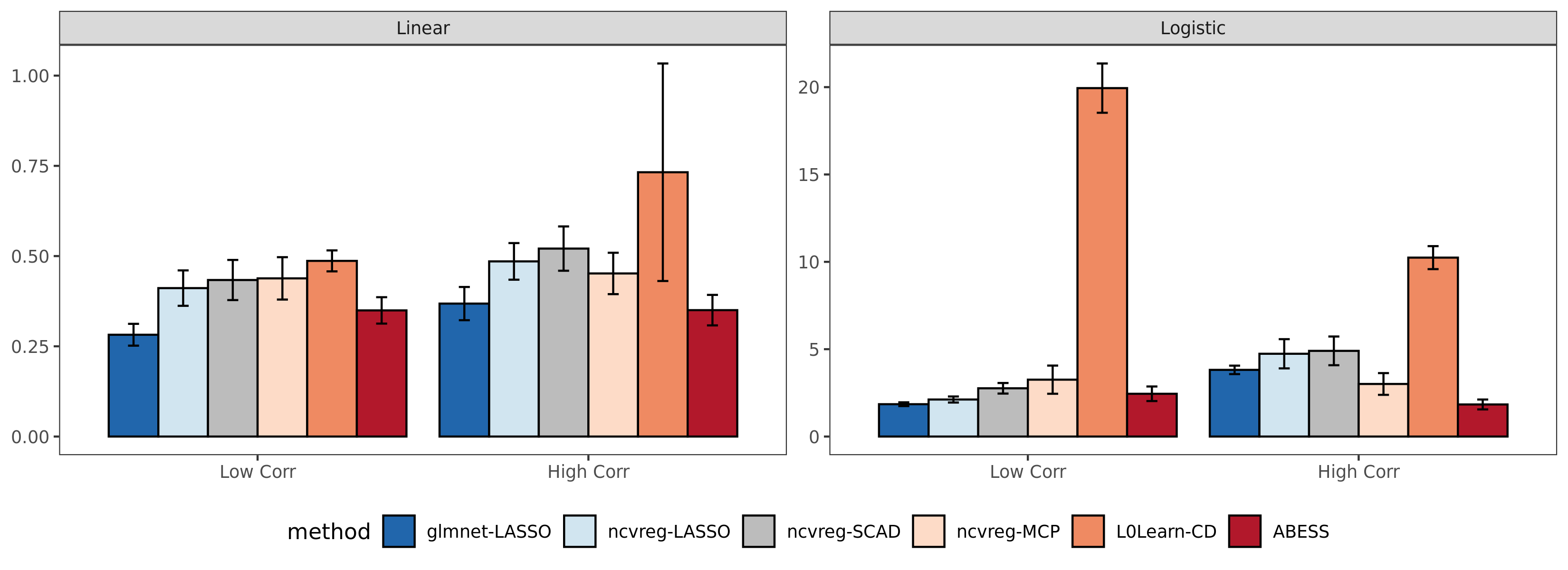
All these packages are compared in three aspects including the prediction performance, the variable selection performance, and the computation efficiency. The prediction performance of the linear model is measured by on a test set and for logistic regression this is measured by the area under the ROC Curve. For the variable selection performance, we compute the true positive rate (TPR, which is the proportion of variables in the active set that are correctly identified) and the false positive rate (FPR, which is the proportion of the variables in the inactive set that are falsely identified as a signal). Timings of the CPU execution are recorded in seconds and all the performances are averaged over 100 replications on a sequence of 100 regularization parameters.
The designed matrix is formed by i.i.d samples generated from a multivariate normal distribution with mean 0 and covariance matrix . We consider two settings—low correlation and high correlation of the predictors. For the low correlation scenario, we set and for the high correlation . The number of predictors is 1000. The true coefficient is a vector with 10 nonzero entries uniformly distributed in . We set , for linear regression , for logistic regression and , for poisson regression. A random noise generated from a standard Gaussian distribution is added to the linear predictor for linear regression. The size of training data for linear regression is 500 and 1000 for logistic regression.
All experiments are evaluated on an Ubuntu system with Intel(R) Core(TM) i9-9940X CPU @ 3.30GHz 3.31 GHz and under R version 3.6.3.
source("docs/simulation/R/timings.R")Results
The results are presented in the following pictures.
First, among all of the methods implemented in different packages, the estimator obtained by the abess package shows the best prediction performance.
Second, the estimator obtained by the abess package can reasonably control the FPR at a low level like SCAD and MCP while preventing the poor true signal detection problem as SCAD and MCP in the linear model when the correlation between predictors is high.
Furthermore, our abess package is highly efficient compared with other packages. To conduct the same task, the abess package is never eclipsed by the glmnet package which is esteemed as the benchmark of efficiency.
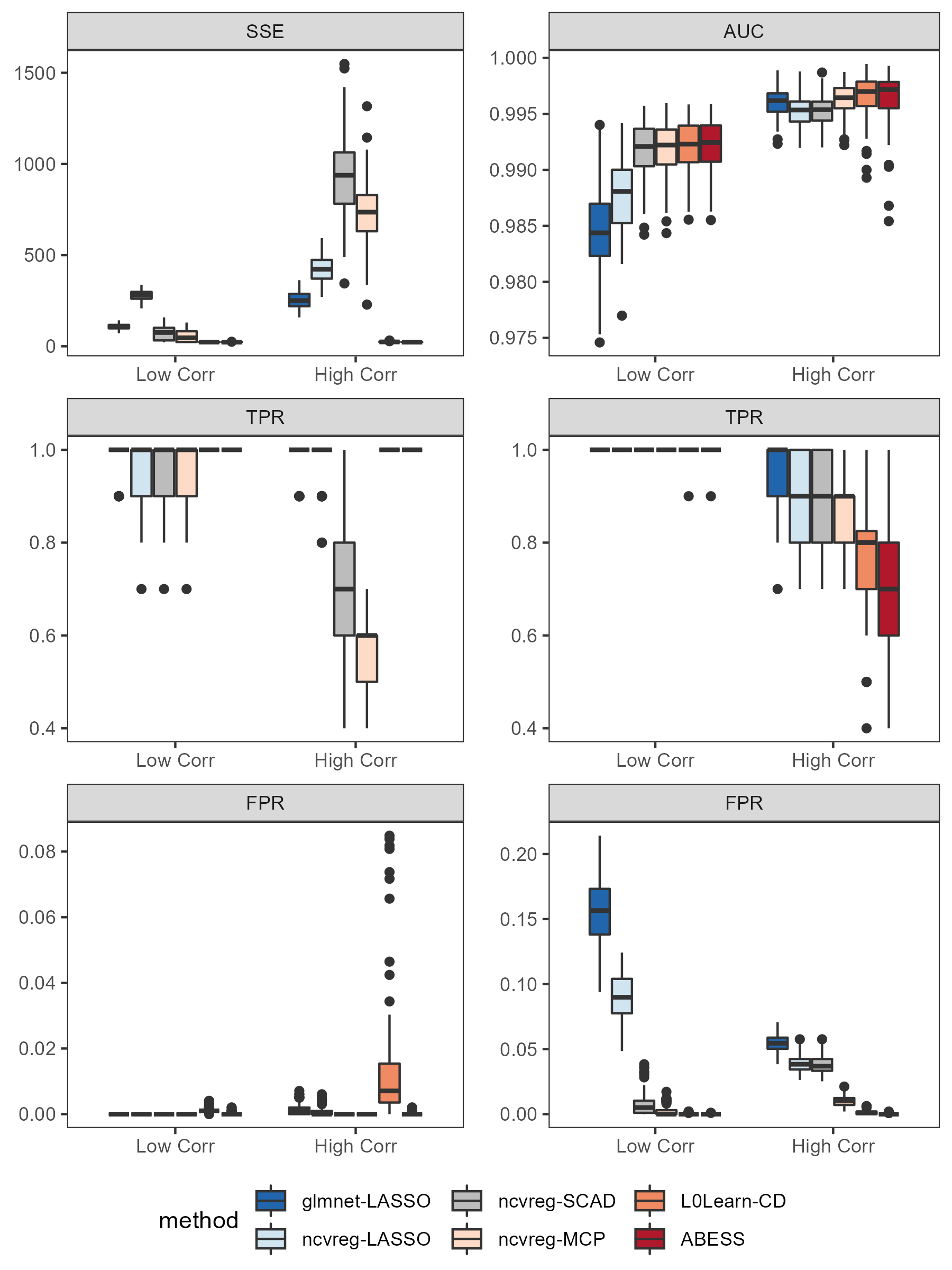
Here we see that the spike-and-slab-prior-based best subset selection estimator meets difficulties in recovering the true active set in logistic regression when the predictors are highly correlated, but still enjoys the best prediction performance. This is that when the predictors are highly correlated, we only need a small subset of predictors to explain the response. For a better variable selection, while maintaining the perfect prediction, a regularized best subset selection is recommended and also available in the abess package. For more information on the regularized best subset selection, please refer to Advanced Features.