Classification: Logistic Regression and Multinomial Extension

Jin Zhu, Liyuan Hu

6/12/2021

Titanic Dataset and Classification

Consider the Titanic dataset obtained from the Kaggle competition: https://www.kaggle.com/c/titanic/data. The dataset consists of data about 889 passengers, and the goal of the competition is to predict the survival (yes/no) based on features including the class of service, the sex, the age etc.

dat <- read.csv('train.csv', header = TRUE, na.strings = c(""))
dim(dat)

## [1] 891  12

head(dat)

##   PassengerId Survived Pclass
## 1           1        0      3
## 2           2        1      1
## 3           3        1      3
## 4           4        1      1
## 5           5        0      3
## 6           6        0      3
##                                                  Name    Sex Age SibSp Parch
## 1                             Braund, Mr. Owen Harris   male  22     1     0
## 2 Cumings, Mrs. John Bradley (Florence Briggs Thayer) female  38     1     0
## 3                              Heikkinen, Miss. Laina female  26     0     0
## 4        Futrelle, Mrs. Jacques Heath (Lily May Peel) female  35     1     0
## 5                            Allen, Mr. William Henry   male  35     0     0
## 6                                    Moran, Mr. James   male  NA     0     0
##             Ticket    Fare Cabin Embarked
## 1        A/5 21171  7.2500  <NA>        S
## 2         PC 17599 71.2833   C85        C
## 3 STON/O2. 3101282  7.9250  <NA>        S
## 4           113803 53.1000  C123        S
## 5           373450  8.0500  <NA>        S
## 6           330877  8.4583  <NA>        Q

Logistic regression is one of powerful tool to tackle this problem. In statistics, the logistic regression is used to model the probability of a certain class or event existing such as alive/dead, pass/fail, win/lose, or healthy/sick. Logistic regression function is an $s$-shaped curve modeling the posterior probability $p$ via a linear combination of the features. The curve is defined as $p = \frac{1}{1+\exp(-\eta)}$ where $\eta = \boldsymbol\beta_0+x\boldsymbol\beta$ and $x$ are predictors, and $\boldsymbol\beta_0, \boldsymbol\beta$ are coefficients to be learned from data. The logistic regression model has this form: $$\log(p/(1-p)) = \boldsymbol\beta_0 + x\boldsymbol\beta.$$ The quantity $\log(p/(1-p))$ is called the logarithm of the odd, also called log-odd or logit. The best subset selection for logistic regression aim to balance model accuracy and model complexity, where the former is achieves by maximizing the log-likelihood function and the latter is characterized by a constraint: $\| \boldsymbol\beta \|_0 \leq s$ and $s$ can be determined in a data driven way.

Best Subset Selection for Logistic Regression

The abess() function in the abess package allows users to perform best subset selection in a highly efficient way. Users can call the abess() function using formula just like what users do with lm(). Or users can specify the design matrix x and the response y. As an example, the Titanic dataset is used to demonstrated the usage of abess package.

Data preprocessing

A glance at the dataset finds there is any missing data. The na.omit() function allows us to delete the rows that contain any missing data. After that, we get a total of 714 samples left.

dat <- na.omit(dat[, c(2, 3, 5, 6, 7, 8, 10, 12)])
dim(dat)

## [1] 712   8

Then we change the factors into dummy variables with the model.matrix() function. Note that the abess function will automatically include the intercept, and thus, we exclude the first column of dat object.

dat <- model.matrix(~., dat)[, -1]
dat <- as.data.frame(dat)

We split the dataset into a training set and a test set. The model is going to be built on the training set and later We will test the model performance on the test set.

train_index <- 1:round((712*2)/3)
train <- dat[train_index, ]
test <- dat[-train_index, ]

Analyze Titanic dataset with abess package

We use abess package to perform best subset selection for the preprocessed Titanic dataset by setting family = "binomial". The cross validation technique is employed to tune the support size by setting tune.type = "cv".

library(abess)
abess_fit <- abess(x = train[, -1], y = train$Survived, 
                   family = "binomial", tune.type = "cv")

After getting the estimator, we can further do more exploring work. The output of abess() function contains the best model for all the candidate support sizes in the support.size. Users can use some generic functions to quickly draw some information of those estimators. Typical examples include:
i. print the fitted model:

abess_fit

## Call:
## abess.default(x = train[, -1], y = train$Survived, family = "binomial", 
##     tune.type = "cv")
## 
##   support.size      dev       cv
## 1            0 321.9560 64.59866
## 2            1 246.5820 49.99585
## 3            2 229.6078 46.65819
## 4            3 224.0843 47.10831
## 5            4 220.4441 45.75501
## 6            5 220.1834 46.31408
## 7            6 220.0022 46.45407
## 8            7 219.9602 46.39656
## 9            8 219.9210 46.44844

2. draw the estimated coefficients on all candidate support size by coef() function:

coef(abess_fit)

## 9 x 9 sparse Matrix of class "dgCMatrix"
##                      0         1          2           3           4           5
## (intercept) -0.3530971  1.158781  2.9213405  4.23196071  4.76830134  4.85381911
## Pclass       .          .        -0.7952709 -1.01705745 -1.03770046 -1.00849770
## Sexmale      .         -2.545075 -2.5818944 -2.51198958 -2.60544822 -2.59656529
## Age          .          .         .         -0.02923674 -0.03712932 -0.03672237
## SibSp        .          .         .          .          -0.36190220 -0.35770273
## Parch        .          .         .          .           .           .         
## Fare         .          .         .          .           .           .         
## EmbarkedQ    .          .         .          .           .           .         
## EmbarkedS    .          .         .          .           .          -0.21507393
##                        6            7            8
## (intercept)  5.112870189  5.106984422  5.079012311
## Pclass      -1.076540803 -1.080872143 -1.085091547
## Sexmale     -2.610618146 -2.600190268 -2.601337076
## Age         -0.037469295 -0.037121587 -0.037259374
## SibSp       -0.339014180 -0.350547546 -0.350406211
## Parch        .            0.048198890  0.053009524
## Fare        -0.001997874 -0.002237775 -0.002224556
## EmbarkedQ    .            .            0.210160985
## EmbarkedS   -0.245382497 -0.255782092 -0.214986232

3. get the deviance of the estimated model on all candidate support sizes via deviance() function:

deviance(abess_fit)

## [1] 321.9560 246.5820 229.6078 224.0843 220.4441 220.1834 220.0022 219.9602
## [9] 219.9210

4. visualize the change of models with the change of support size via plot() function:

plot(abess_fit, label=T)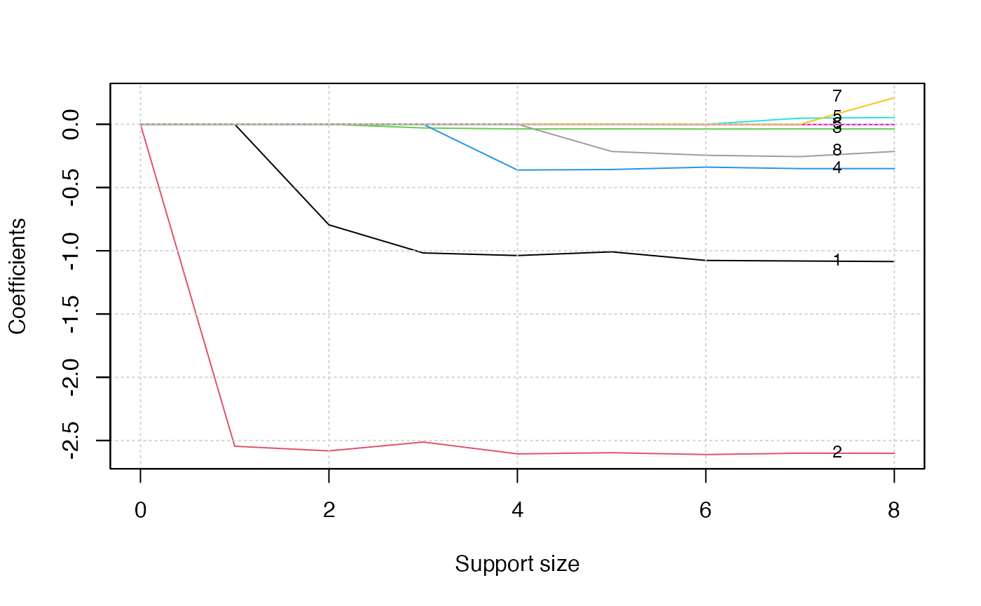

The graph shows that, beginning from the most dense model, the second variable (Sex) is included in the active set until the support size reaches 0. We can also generate a graph about the tuning value.

plot(abess_fit, type = "tune")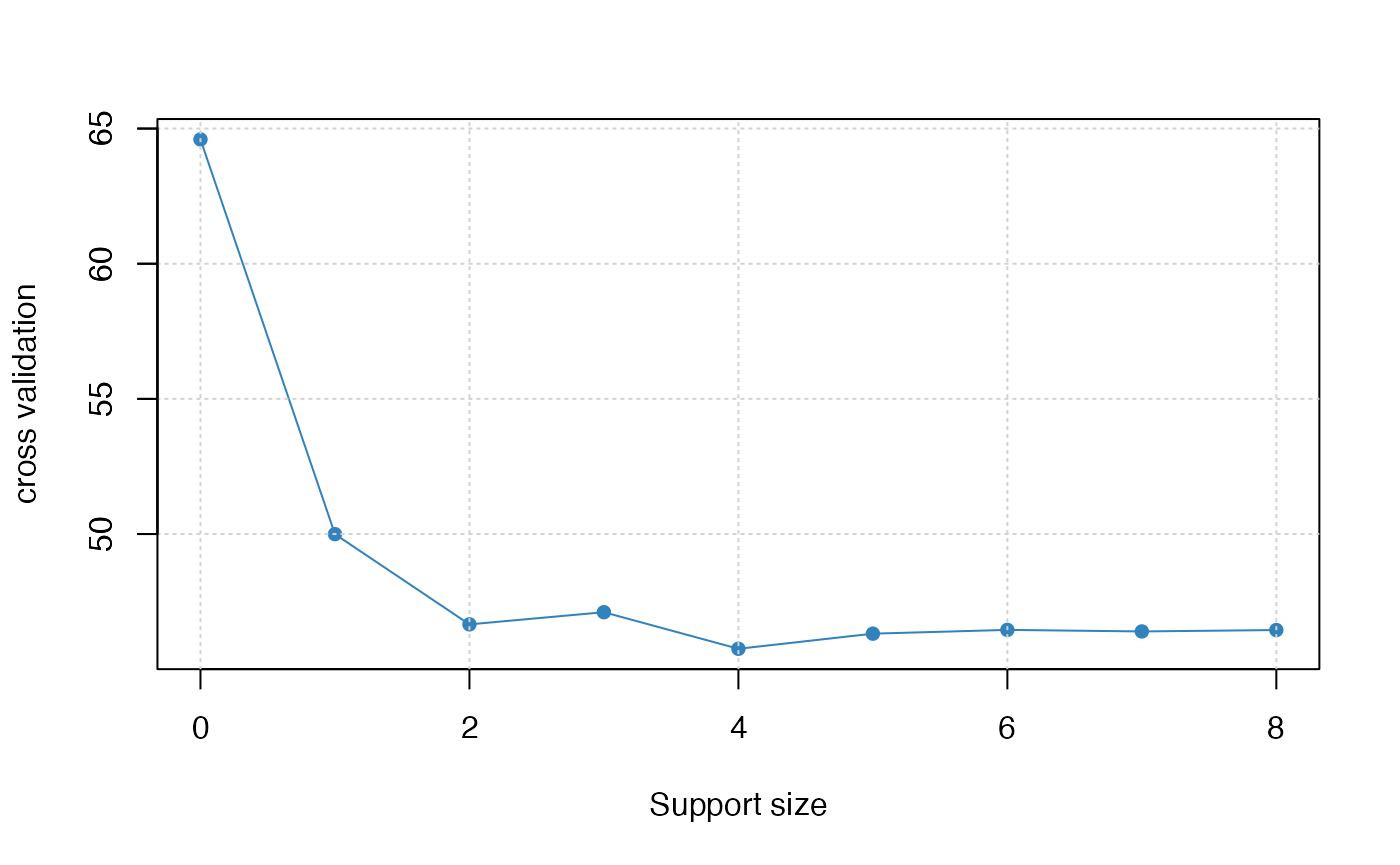

The tuning value reaches the lowest point at 4, which implies the best model consists of four variables.

Finally, to extract the specified model from the abess object, we can call the extract() function with a given support.size. If support.size is not provided, the model with the best tuning value will be returned. Here we extract the model with support size equals 6.

best.model <- extract(abess_fit, support.size = 4)
str(best.model)

## List of 7
##  $ beta        :Formal class 'dgCMatrix' [package "Matrix"] with 6 slots
##   .. ..@ i       : int [1:4] 0 1 2 3
##   .. ..@ p       : int [1:2] 0 4
##   .. ..@ Dim     : int [1:2] 8 1
##   .. ..@ Dimnames:List of 2
##   .. .. ..$ : chr [1:8] "Pclass" "Sexmale" "Age" "SibSp" ...
##   .. .. ..$ : chr "4"
##   .. ..@ x       : num [1:4] -1.0377 -2.6054 -0.0371 -0.3619
##   .. ..@ factors : list()
##  $ intercept   : num 4.77
##  $ support.size: num 4
##  $ support.vars: chr [1:4] "Pclass" "Sexmale" "Age" "SibSp"
##  $ support.beta: num [1:4] -1.0377 -2.6054 -0.0371 -0.3619
##  $ dev         : num 220
##  $ tune.value  : num 45.8

The return is a list containing the basic information of the estimated model.

Make a Prediction

Prediction is allowed for all the estimated models. Just call predict.abess() function with the support.size set to the size of model users are interested in. If support.size is not provided, prediction will be made based on the best tuning value. The predict.abess() can provide both link, standing for the linear predictors, and the response, standing for the fitted probability. Here We will predict the probability of survival on the test.csv data.

fitted.results <- predict(abess_fit, newx = test, type = 'response')

If we chose 0.5 as the cut point, i.e, we predict the person survives the sinking of the Titanic if the fitted probability is greater than 0.5, the accuracy will be 0.80.

fitted.results <- ifelse(fitted.results > 0.5, 1, 0)
misClasificError <- mean(fitted.results != test$Survived)
print(paste('Accuracy',1-misClasificError))

## [1] "Accuracy 0.79746835443038"

We can also generate an ROC and calculate the AUC value. On this dataset, the AUC is 0.87, which is quite close to 1.

library(ROCR)
fitted.results <- predict(abess_fit, newx = test, type = 'response')
pr <- prediction(fitted.results, test$Survived)
prf <- performance(pr, measure = "tpr", x.measure = "fpr")
plot(prf)

auc <- performance(pr, measure = "auc")
auc <- auc@y.values[[1]]
auc

## [1] 0.8739505

Extension: Multi-class Classification

Best subset selection for multinomial logistic regression

When the number of classes is more than 2, we call it multi-class classification task. Logistic regression can be extended to model several classes of events such as determining whether an image contains a cat, dog, lion, etc. Each object detected in the image would be assigned a probability between 0 and 1, with a sum of one. The extended model is multinomial logistic regression.

To arrive at the multinomial logistic model, one can imagine, for $K$ possible classes, running $K-1$ independent logistic regression models, in which one class is chosen as a ``pivot’’ and then the other $K-1$ classes are separately regressed against the pivot outcome. This would proceed as follows, if class K (the last outcome) is chosen as the pivot: $$\ln(\mathbb{P}(y = 1) / \mathbb{P}(y = K)) = x^\top \boldsymbol\beta^{(1)},$$$$\cdots \cdots$$$$\ln(\mathbb{P}(y = K - 1) / \mathbb{P}(y = K)) = x^\top \boldsymbol\beta^{(K - 1)}.$$ Then, the probability to choose the $j$-th class can be easily derived to be: $$\mathbb{P}(y = j) = \frac{\exp{(x^\top \boldsymbol\beta^{(j)})}}{1 + \sum_{k=1}^{K-1} \exp{(x^\top \boldsymbol\beta^{(k)})}},$$ and subsequently, we would predict the $j^{*}$-th class if the $j^* = \arg\max_{j} \mathbb{P}(y = j)$. Notice that, for $K$ possible classes case, there are $p \times (K - 1)$ unknown parameters: $\boldsymbol\beta^{(1)}, \ldots, \boldsymbol\beta^{(K-1)}$ to be estimated. Because the number of parameters increase as $K$, it is even more urge to constrain the model complexity. And the best subset selection for multinomial logistic regression aims to maximize the log-likelihood function and control the model complexity by restricting $B = (\boldsymbol\beta^{(1)}, \ldots, \boldsymbol\beta^{(K-1)})$ with $\| B \|_{0, 2} \leq s$ where $\| B \|_{0, 2} = \sum_{i = 1}^{p} I(B_{i\cdot} = {\bf 0})$, $B_{i\cdot}$ is the $i$-th row of coefficient matrix $B$ and ${\bf 0} \in R^{K - 1}$ is an all zero vector. In other words, each row of $B$ would be either all zero or all non-zero.

Multinomial logistic regression with abess Package

We shall conduct Multinomial logistic regression on an artificial dataset for demonstration. The generate.data() function provides a simple way to generate suitable for this task. The assumption behind is the response vector following a multinomial distribution. The artifical dataset contain 100 observations and 20 predictors but only five predictors have influence on the three possible classes.

library(abess)
n <- 100
p <- 20
support.size <- 5
dataset <- generate.data(n, p, support.size, family = "multinomial", class.num = 3)
head(dataset$y)

## [1] 1 2 1 1 0 0

dataset$beta

##            [,1]      [,2]      [,3]
##  [1,]  0.000000  0.000000  0.000000
##  [2,]  0.000000  0.000000  0.000000
##  [3,]  0.000000  0.000000  0.000000
##  [4,]  0.000000  0.000000  0.000000
##  [5,]  0.000000  0.000000  0.000000
##  [6,] 16.244248  6.605285  4.958967
##  [7,]  0.000000  0.000000  0.000000
##  [8,]  0.000000  0.000000  0.000000
##  [9,]  0.000000  0.000000  0.000000
## [10,]  0.000000  0.000000  0.000000
## [11,]  3.462001  6.774016 20.454220
## [12,]  0.000000  0.000000  0.000000
## [13,] 18.987979 13.133145 17.211335
## [14,]  8.034160  1.117907  2.904334
## [15,]  0.000000  0.000000  0.000000
## [16,]  0.000000  0.000000  0.000000
## [17,]  0.000000  0.000000  0.000000
## [18,] 23.307996 17.576156 11.922882
## [19,]  0.000000  0.000000  0.000000
## [20,]  0.000000  0.000000  0.000000

To carry out best subset selection for multinomial logistic regression, users can call the abess() function with family specified to multinomial. Here is an example.

abess_fit <- abess(dataset[["x"]], dataset[["y"]], 
                   family = "multinomial", tune.type = "cv")
extract(abess_fit)[["support.vars"]]

## [1] "x6"  "x11" "x13" "x14" "x18"

Notice that the abess() correctly identifies the support set of the ground truth coefficient matrix.