Advanced Features

Introduction

When analyzing the real world datasets, we may have the following targets:
1. certain variables must be selected when some prior information is given;
2. selecting the weak signal variables when the prediction performance is main interest;
3. identifying predictors when group structure are provided;
4. pre-excluding a part of predictors when datasets have ultra high-dimensional predictors.

In the following content, we will illustrate the statistic methods to reach these targets in a one-by-one manner, and give quick examples to show how to perform the statistic methods with the abess package. Actually, in the abess package, there targets can be properly handled by simply change the default arguments in the abess() function.

Nuisance Regression

Nuisance regression refers to best subset selection with some prior information that some variables are required to stay in the active set. For example, if we are interested in a certain gene and want to find out what other genes are associated with the response when this particular gene shows effect.

Carrying Out the Nuisance Regression with abess

In the abess() function, the argument always.include is designed to realize this goal. user can pass a vector containing the indexes of the target variables to always.include. Here is an example.

library(abess)

## 
##  Thank you for using abess! To acknowledge our work, please cite the package:

## 
##  Zhu J, Wang X, Hu L, Huang J, Jiang K, Zhang Y, Lin S, Zhu J (2022). 'abess: A Fast Best Subset Selection Library in Python and R.' Journal of Machine Learning Research, 23(202), 1-7. https://www.jmlr.org/papers/v23/21-1060.html.

n <- 100
p <- 20
support.size <- 3
dataset <- generate.data(n, p, support.size)
dataset$beta

##  [1]  0.00000  0.00000  0.00000  0.00000  0.00000 84.67713  0.00000  0.00000
##  [9]  0.00000  0.00000  0.00000  0.00000  0.00000 85.82187  0.00000  0.00000
## [17]  0.00000 47.40922  0.00000  0.00000

abess_fit <- abess(dataset[["x"]], dataset[["y"]], always.include = 6)
coef(abess_fit, support.size = abess_fit$support.size[which.min(abess_fit$tune.value)])

## 21 x 1 sparse Matrix of class "dgCMatrix"
##                      4
## (intercept)  -4.767241
## x1            .       
## x2            .       
## x3            .       
## x4            .       
## x5            .       
## x6           82.424118
## x7            .       
## x8            .       
## x9            .       
## x10           .       
## x11           .       
## x12           .       
## x13           .       
## x14          89.031689
## x15           .       
## x16         -12.622583
## x17           .       
## x18          43.343247
## x19           .       
## x20           .

Regularized Adaptive Best Subset Selection

In some cases, especially under low signal-to-noise ratio (SNR) setting or predictors are highly correlated, the vanilla type of \(L_0\) constrained model may not be satisfying and a more sophisticated trade-off between bias and variance is needed. Under this concern, the abess package provides option of best subset selection with \(L_2\) norm regularization called the regularized best subset selection (BESS). The model has this following form:

\[\begin{align} \min_{\boldsymbol\beta} \mathcal{L_n}({\boldsymbol\beta}) + \lambda \|\boldsymbol\beta\|_2^2. \end{align}\]

Carrying out the Regularized BESS

To implement the regularized BESS, user need to specify a value to the lambda in the abess() function. This lambda value corresponds to the penalization parameter in the model above. Here we give an example.

library(abess)
n <- 100
p <- 30
snr <- 0.05
dataset <- generate.data(n, p, snr = snr, seed = 1, beta = rep(c(1, rep(0 ,5)), each = 5), rho = 0.8, cortype = 3)
data.test <- generate.data(n, p, snr = snr, beta = dataset$beta, seed = 100)
abess_fit <- abess(dataset[["x"]], dataset[["y"]], lambda = 0.7)

Let’s test the regularized best subset selection against the no-regularized one over 100 replications in terms of prediction performance.

M <- 100
err.l0 <- rep(0, M)
err.l0l2 <- rep(0, M)
for(i in 1:M){
  dataset <- generate.data(n, p, snr = snr, seed = i, beta = rep(c(1, rep(0 ,5)), each = 5), rho = 0.8, cortype = 3)
  data.test <- generate.data(n, p, snr = snr, beta = dataset$beta, seed = i+100)
  
  abess_fit <- abess(dataset[["x"]], dataset[["y"]], lambda = 0.7)
  coef(abess_fit, support.size = abess_fit$support.size[which.min(abess_fit$tune.value)])
  pe.l0l2 <-  norm(data.test$y - predict(abess_fit, newx = data.test$x),'2')
  err.l0[i] <- pe.l0l2
  
  abess_l0 <- abess(dataset[["x"]], dataset[["y"]])
  coef(abess_l0, support.size = abess_l0$support.size[which.min(abess_l0$tune.value)])
  pe.l0 <- norm(data.test$y -predict(abess_l0, newx = data.test$x), '2')
  err.l0l2[i] <- pe.l0
}
mean(err.l0)

## [1] 133.4154

mean(err.l0l2)

## [1] 152.979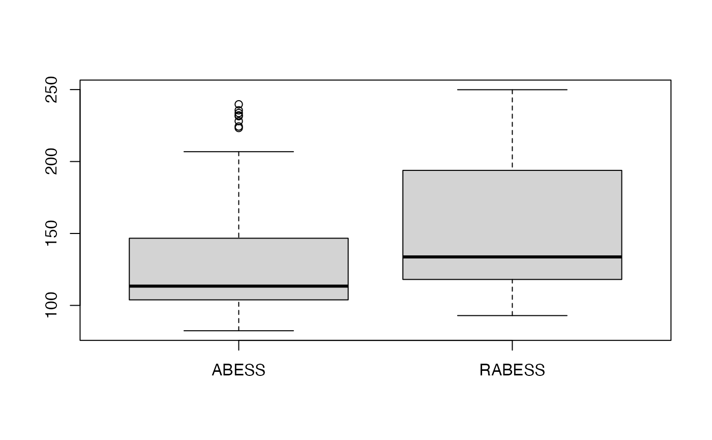1

boxplot(list("ABESS" = err.l0, "RABESS" = err.l0l2))

We see that the regularized best subset select indeed reduces the prediction error.

Best group subset selection

Group linear model is a linear model which the \(p\) predictors are separated into \(J\) pre-determined non-overlapping groups,

\[ y = \sum_{j=1}^J X_{G_j} \boldsymbol{\beta_{G_j}}+\epsilon, \] where \(\{G_j\}_{j=1}^J\) are the group indices of the \(p\) predictors.

Best group subset selection (BGSS) aims to choose a small part of groups to achieve the best interpretability on the response variable. BGSS is practically useful for the analysis of variables with certain group structures.

The BGSS can be achieved by solving: \[\begin{equation}\label{eq:constraint} \min\limits_{\beta \in \mathbb{R}^p} \mathcal{L_n}({\boldsymbol\beta}),\quad s.t.\ \|\boldsymbol{\beta}\|_{0,2}\leqslant s, \end{equation}\] where the \(\ell_{0,2}\) (-pseudo) norm is defined as \(\|{{\boldsymbol\beta}}\|_{0,2} = \sum_{j=1}^J \mathrm{I} (\|\boldsymbol{\beta_{G_j}}\|_2 \neq 0)\) and model size \(s\) is a positive integer to be determined from data. Regardless of the NP-hard of this problem, Zhang et al develop a certifiably polynomial algorithm with a high probability to solve it. This algorithm is integrated in the abess package, and user can handily select best group subset by assigning a proper value to the group.index arguments in abess() function.

Quick example

We use a synthetic dataset to demonstrate its usage. The dataset consists of 100 observations. Each observation has 20 predictors but only the first three predictors among them have a impact on the response.

set.seed(1234)
n <- 100
p <- 20
support.size <- 3
dataset <- generate.data(n, p, beta = c(10, 5, 5, rep(0, 17)))

Supposing we have some prior information that the second and third variables belong to the same group, then we can set the group_index as:

group_index <- c(1, 2, 2, seq(3, 19, by = 1))

Then, pass this group_index to the abess() function:

abess_fit <- abess(dataset[["x"]], dataset[["y"]], 
                   group.index = group_index)
str(extract(abess_fit))

## List of 7
##  $ beta        :Formal class 'dgCMatrix' [package "Matrix"] with 6 slots
##   .. ..@ i       : int [1:3] 0 1 2
##   .. ..@ p       : int [1:2] 0 3
##   .. ..@ Dim     : int [1:2] 20 1
##   .. ..@ Dimnames:List of 2
##   .. .. ..$ : chr [1:20] "x1" "x2" "x3" "x4" ...
##   .. .. ..$ : chr "2"
##   .. ..@ x       : num [1:3] 10.2 4.92 4.88
##   .. ..@ factors : list()
##  $ intercept   : num 0.0859
##  $ support.size: int 2
##  $ support.vars: chr [1:3] "x1" "x2" "x3"
##  $ support.beta: num [1:3] 10.2 4.92 4.88
##  $ dev         : num 8.3
##  $ tune.value  : num 225

The fitted result suggest that only two groups are selected (since support.size is 2) and the selected variables are matched with the ground truth setting.

Feature screening

In the case of ultra high-dimensional data, it is more effective to do feature screening first before carrying out feature selection. The abess package allowed users to perform the sure independent screening to pre-exclude some features according to the marginal likelihood.

Integrate SIS in `abess` package

Ultra-high dimensional predictors increase computational cost but reduce estimation accuracy for any statistical procedure. To reduce dimensionality from high to a relatively acceptable level, a fairly general asymptotic framework, named feature screening (sure independence screening) is proposed to tackle even exponentially growing dimension. The feature screening can theoretically maintain all effective predictors with a high probability, which is called the sure screening property. In the abess() function, to carrying out the Integrate SIS, user need to passed an integer smaller than the number of the predictors to the screening.num. Then the abess() function will first calculate the marginal likelihood of each predictor and reserve those predictors with the screening.num largest marginal likelihood. Then, the ABESS algorithm is conducted only on this screened subset. Here is an example.

library(abess)
n <- 100
p <- 1000
support.size <- 3
dataset <- generate.data(n, p, support.size)
abess_fit <- abess(dataset[["x"]], dataset[["y"]], 
                   screening.num = 100)

Jin Zhu, Yanhang Zhang

1/21/2022

Introduction

Nuisance Regression

Carrying Out the Nuisance Regression with abess

Regularized Adaptive Best Subset Selection

Carrying out the Regularized BESS

Best group subset selection

Quick example

Feature screening

Integrate SIS in `abess` package

Advanced Features

Jin Zhu, Yanhang Zhang

1/21/2022

Introduction

Nuisance Regression

Carrying Out the Nuisance Regression with abess

Regularized Adaptive Best Subset Selection

Carrying out the Regularized BESS

Best group subset selection

Quick example

Feature screening

Integrate SIS in abess package

Integrate SIS in `abess` package