Adaptive best-subset selection for regression, (multi-class) classification, counting-response, censored-response, positive response, multi-response modeling in polynomial times.
# Default S3 method
abess(
  x,
  y,
  family = c("gaussian", "binomial", "poisson", "cox", "mgaussian", "multinomial",
    "gamma", "ordinal"),
  tune.path = c("sequence", "gsection"),
  tune.type = c("gic", "ebic", "bic", "aic", "cv"),
  weight = NULL,
  normalize = NULL,
  fit.intercept = TRUE,
  beta.low = -.Machine$double.xmax,
  beta.high = .Machine$double.xmax,
  c.max = 2,
  support.size = NULL,
  gs.range = NULL,
  lambda = 0,
  always.include = NULL,
  group.index = NULL,
  init.active.set = NULL,
  splicing.type = 2,
  max.splicing.iter = 20,
  screening.num = NULL,
  important.search = NULL,
  warm.start = TRUE,
  nfolds = 5,
  foldid = NULL,
  cov.update = FALSE,
  newton = c("exact", "approx"),
  newton.thresh = 1e-06,
  max.newton.iter = NULL,
  early.stop = FALSE,
  ic.scale = 1,
  num.threads = 0,
  seed = 1,
  ...
)

# S3 method for class 'formula'
abess(formula, data, subset, na.action, ...)
Arguments
- x
Input matrix, of dimension \(n \times p\); each row is an observation vector and each column is a predictor/feature/variable. Can be in sparse matrix format (inherit from class
"dgCMatrix"in packageMatrix).- y
The response variable, of
nobservations. Forfamily = "binomial"should have two levels. Forfamily="poisson",yshould be a vector with positive integer. Forfamily = "cox",yshould be aSurvobject returned by thesurvivalpackage (recommended) or a two-column matrix with columns named"time"and"status". Forfamily = "mgaussian",yshould be a matrix of quantitative responses. Forfamily = "multinomial"or"ordinal",yshould be a factor of at least three levels. Note that, for either"binomial","ordinal"or"multinomial", if y is presented as a numerical vector, it will be coerced into a factor.- family
One of the following models:
"gaussian"(continuous response),"binomial"(binary response),"poisson"(non-negative count),"cox"(left-censored response),"mgaussian"(multivariate continuous response),"multinomial"(multi-class response),"ordinal"(multi-class ordinal response),"gamma"(positive continuous response). Depending on the response. Any unambiguous substring can be given.- tune.path
The method to be used to select the optimal support size. For
tune.path = "sequence", we solve the best subset selection problem for each size insupport.size. Fortune.path = "gsection", we solve the best subset selection problem with support size ranged ings.range, where the specific support size to be considered is determined by golden section.- tune.type
The type of criterion for choosing the support size. Available options are
"gic","ebic","bic","aic"and"cv". Default is"gic".- weight
Observation weights. When
weight = NULL, we setweight = 1for each observation as default.- normalize
Options for normalization.
normalize = 0for no normalization.normalize = 1for subtracting the means of the columns ofxandy, and also normalizing the columns ofxto have \(\sqrt n\) norm.normalize = 2for subtracting the mean of columns ofxand scaling the columns ofxto have \(\sqrt n\) norm.normalize = 3for scaling the columns ofxto have \(\sqrt n\) norm. Ifnormalize = NULL,normalizewill be set1for"gaussian"and"mgaussian",3for"cox". Default isnormalize = NULL.- fit.intercept
A boolean value indicating whether to fit an intercept. We assume the data has been centered if
fit.intercept = FALSE. Default:fit.intercept = TRUE.- beta.low
A single value specifying the lower bound of \(\beta\). Default is
-.Machine$double.xmax.- beta.high
A single value specifying the upper bound of \(\beta\). Default is
.Machine$double.xmax.- c.max
an integer splicing size. Default is:
c.max = 2.- support.size
An integer vector representing the alternative support sizes. Only used for
tune.path = "sequence". Default is0:min(n, round(n/(log(log(n))log(p)))).- gs.range
A integer vector with two elements. The first element is the minimum model size considered by golden-section, the later one is the maximum one. Default is
gs.range = c(1, min(n, round(n/(log(log(n))log(p))))).- lambda
A single lambda value for regularized best subset selection. Default is 0.
- always.include
An integer vector containing the indexes of variables that should always be included in the model.
- group.index
A vector of integers indicating the which group each variable is in. For variables in the same group, they should be located in adjacent columns of
xand their corresponding index ingroup.indexshould be the same. Denote the first group as1, the second2, etc. If you do not fit a model with a group structure, please setgroup.index = NULL(the default).- init.active.set
A vector of integers indicating the initial active set. Default:
init.active.set = NULL.- splicing.type
Optional type for splicing. If
splicing.type = 1, the number of variables to be spliced isc.max, ...,1; ifsplicing.type = 2, the number of variables to be spliced isc.max,c.max/2, ...,1. (Default:splicing.type = 2.)- max.splicing.iter
The maximum number of performing splicing algorithm. In most of the case, only a few times of splicing iteration can guarantee the convergence. Default is
max.splicing.iter = 20.- screening.num
An integer number. Preserve
screening.numnumber of predictors with the largest marginal maximum likelihood estimator before running algorithm.- important.search
An integer number indicating the number of important variables to be splicing. When
important.search\(\ll\)pvariables, it would greatly reduce runtimes. Default:important.search = 128.- warm.start
Whether to use the last solution as a warm start. Default is
warm.start = TRUE.- nfolds
The number of folds in cross-validation. Default is
nfolds = 5.- foldid
an optional integer vector of values between 1, ..., nfolds identifying what fold each observation is in. The default
foldid = NULLwould generate a random foldid.- cov.update
A logical value only used for
family = "gaussian". Ifcov.update = TRUE, use a covariance-based implementation; otherwise, a naive implementation. The naive method is more computational efficient than covariance-based method when \(p >> n\) andimportant.searchis much large than its default value. Default:cov.update = FALSE.- newton
A character specify the Newton's method for fitting generalized linear models, it should be either
newton = "exact"ornewton = "approx". Ifnewton = "exact", then the exact hessian is used, whilenewton = "approx"uses diagonal entry of the hessian, and can be faster (especially whenfamily = "cox").- newton.thresh
a numeric value for controlling positive convergence tolerance. The Newton's iterations converge when \(|dev - dev_{old}|/(|dev| + 0.1)<\)
newton.thresh.- max.newton.iter
a integer giving the maximal number of Newton's iteration iterations. Default is
max.newton.iter = 10ifnewton = "exact", andmax.newton.iter = 60ifnewton = "approx".- early.stop
A boolean value decide whether early stopping. If
early.stop = TRUE, algorithm will stop if the last tuning value less than the existing one. Default:early.stop = FALSE.- ic.scale
A non-negative value used for multiplying the penalty term in information criterion. Default:
ic.scale = 1.- num.threads
An integer decide the number of threads to be concurrently used for cross-validation (i.e.,
tune.type = "cv"). Ifnum.threads = 0, then all of available cores will be used. Default:num.threads = 0.- seed
Seed to be used to divide the sample into cross-validation folds. Default is
seed = 1.- ...
further arguments to be passed to or from methods.
- formula
an object of class "
formula": a symbolic description of the model to be fitted. The details of model specification are given in the "Details" section of "formula".- data
a data frame containing the variables in the
formula.- subset
an optional vector specifying a subset of observations to be used.
- na.action
a function which indicates what should happen when the data contain
NAs. Defaults togetOption("na.action").
Value
A S3 abess class object, which is a list with the following components:
- beta
A \(p\)-by-
length(support.size)matrix of coefficients for univariate family, stored in column format; while a list oflength(support.size)coefficients matrix (with size \(p\)-by-ncol(y)) for multivariate family.- intercept
An intercept vector of length
length(support.size)for univariate family; while a list oflength(support.size)intercept vector (with sizencol(y)) for multivariate family.- dev
the deviance of length
length(support.size).- tune.value
A value of tuning criterion of length
length(support.size).- nobs
The number of sample used for training.
- nvars
The number of variables used for training.
- family
Type of the model.
- tune.path
The path type for tuning parameters.
- support.size
The actual
support.sizevalues used. Note that it is not necessary the same as the input if the later have non-integer values or duplicated values.- edf
The effective degree of freedom. It is the same as
support.sizewhenlambda = 0.- best.size
The best support size selected by the tuning value.
- tune.type
The criterion type for tuning parameters.
- tune.path
The strategy for tuning parameters.
- screening.vars
The character vector specify the feature selected by feature screening. It would be an empty character vector if
screening.num = 0.- call
The original call to
abess.
Details
Best-subset selection aims to find a small subset of predictors,
so that the resulting model is expected to have the most desirable prediction accuracy.
Best-subset selection problem under the support size \(s\) is
$$\min_\beta -2 \log L(\beta) \;\;{\rm s.t.}\;\; \|\beta\|_0 \leq s,$$
where \(L(\beta)\) is arbitrary convex functions. In
the GLM case, \(\log L(\beta)\) is the log-likelihood function; in the Cox
model, \(\log L(\beta)\) is the log partial-likelihood function.
The best subset selection problem is solved by the splicing algorithm in this package, see Zhu (2020) for details.
Under mild conditions, the algorithm exactly solve this problem in polynomial time.
This algorithm exploits the idea of sequencing and splicing to reach a stable solution in finite steps when \(s\) is fixed.
The parameters c.max, splicing.type and max.splicing.iter allow user control the splicing technique flexibly.
On the basis of our numerical experiment results, we assign properly parameters to the these parameters as the default
such that the precision and runtime are well balanced, we suggest users keep the default values unchanged.
Please see this online page for more details about the splicing algorithm.
To find the optimal support size \(s\),
we provide various criterion like GIC, AIC, BIC and cross-validation error to determine it.
More specifically, the sequence of models implied by support.size are fit by the splicing algorithm.
And the solved model with least information criterion or cross-validation error is the optimal model.
The sequential searching for the optimal model is somehow time-wasting.
A faster strategy is golden section (GS), which only need to specify gs.range.
More details about GS is referred to Zhang et al (2021).
It is worthy to note that the parameters newton, max.newton.iter and newton.thresh allows
user control the parameter estimation in non-gaussian models.
The parameter estimation procedure use Newton method or approximated Newton method (only consider the diagonal elements in the Hessian matrix).
Again, we suggest to use the default values unchanged because the same reason for the parameter c.max.
abess support some well-known advanced statistical methods to analyze data, including
sure independent screening: helpful for ultra-high dimensional predictors (i.e., \(p \gg n\)). Use the parameter
screening.numto retain the marginally most important predictors. See Fan et al (2008) for more details.best subset of group selection: helpful when predictors have group structure. Use the parameter
group.indexto specify the group structure of predictors. See Zhang et al (2021) for more details.\(l_2\) regularization best subset selection: helpful when signal-to-ratio is relatively small. Use the parameter
lambdato control the magnitude of the regularization term.nuisance selection: helpful when the prior knowledge of important predictors is available. Use the parameter
always.includeto retain the important predictors.
The arbitrary combination of the four methods are definitely support.
Please see online vignettes for more details about the advanced features support by abess.
References
A polynomial algorithm for best-subset selection problem. Junxian Zhu, Canhong Wen, Jin Zhu, Heping Zhang, Xueqin Wang. Proceedings of the National Academy of Sciences Dec 2020, 117 (52) 33117-33123; doi:10.1073/pnas.2014241117
A Splicing Approach to Best Subset of Groups Selection. Zhang, Yanhang, Junxian Zhu, Jin Zhu, and Xueqin Wang (2023). INFORMS Journal on Computing, 35:1, 104-119. doi:10.1287/ijoc.2022.1241
abess: A Fast Best-Subset Selection Library in Python and R. Zhu Jin, Xueqin Wang, Liyuan Hu, Junhao Huang, Kangkang Jiang, Yanhang Zhang, Shiyun Lin, and Junxian Zhu. Journal of Machine Learning Research 23, no. 202 (2022): 1-7.
Sure independence screening for ultrahigh dimensional feature space. Fan, J. and Lv, J. (2008), Journal of the Royal Statistical Society: Series B (Statistical Methodology), 70: 849-911. doi:10.1111/j.1467-9868.2008.00674.x
Targeted Inference Involving High-Dimensional Data Using Nuisance Penalized Regression. Qiang Sun & Heping Zhang (2020). Journal of the American Statistical Association, doi:10.1080/01621459.2020.1737079
See also
Examples
# \donttest{
library(abess)
Sys.setenv("OMP_THREAD_LIMIT" = 2)
n <- 100
p <- 20
support.size <- 3
################ linear model ################
dataset <- generate.data(n, p, support.size)
abess_fit <- abess(dataset[["x"]], dataset[["y"]])
## helpful generic functions:
print(abess_fit)
#> Call:
#> abess.default(x = dataset[["x"]], y = dataset[["y"]])
#>
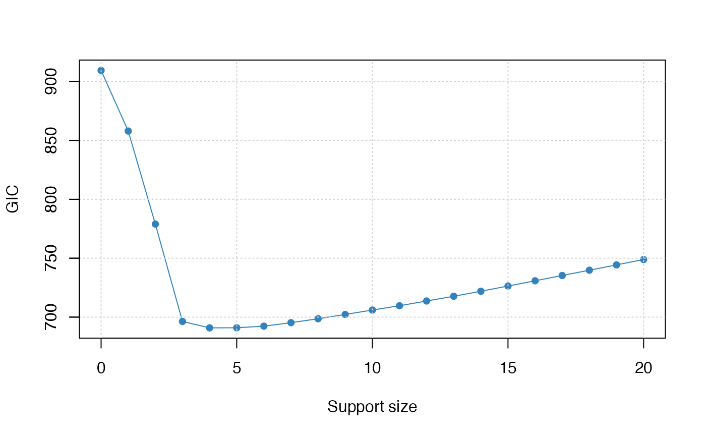
#> support.size dev GIC
#> 1 0 8902.8419 909.4126
#> 2 1 5081.6351 857.9139
#> 3 2 2203.6977 778.9392
#> 4 3 921.3726 696.3115
#> 5 4 833.5074 690.8643
#> 6 5 797.0079 690.9616
#> 7 6 771.9370 692.3404
#> 8 7 759.3075 695.2658
#> 9 8 750.0559 698.6149
#> 10 9 743.0171 702.2471
#> 11 10 736.8746 705.9920
#> 12 11 730.2053 709.6578
#> 13 12 726.1450 713.6752
#> 14 13 722.1120 717.6933
#> 15 14 719.8878 721.9598
#> 16 15 718.7611 726.3782
#> 17 16 717.9167 730.8357
#> 18 17 717.2695 735.3205
#> 19 18 716.6929 739.8151
#> 20 19 716.1755 744.3179
#> 21 20 716.1127 748.8842
coef(abess_fit, support.size = 3)
#> 21 x 1 sparse Matrix of class "dgCMatrix"
#> 3
#> (intercept) -4.369861
#> x1 .
#> x2 .
#> x3 .
#> x4 .
#> x5 .
#> x6 83.270800
#> x7 .
#> x8 .
#> x9 .
#> x10 .
#> x11 .
#> x12 .
#> x13 .
#> x14 89.689944
#> x15 .
#> x16 .
#> x17 .
#> x18 43.410846
#> x19 .
#> x20 .
predict(abess_fit,
newx = dataset[["x"]][1:10, ],
support.size = c(3, 4)
)
#> 3 4
#> [1,] 103.05157 91.524774
#> [2,] 74.66998 85.359664
#> [3,] -289.97309 -299.858907
#> [4,] -16.35758 -4.241221
#> [5,] 171.80572 162.807112
#> [6,] 126.58540 127.021354
#> [7,] -197.24366 -207.134508
#> [8,] -126.67823 -142.927367
#> [9,] -23.29128 -22.898065
#> [10,] -109.76937 -117.273626
str(extract(abess_fit, 3))
#> List of 7
#> $ beta :Formal class 'dgCMatrix' [package "Matrix"] with 6 slots
#> .. ..@ i : int [1:3] 5 13 17
#> .. ..@ p : int [1:2] 0 3
#> .. ..@ Dim : int [1:2] 20 1
#> .. ..@ Dimnames:List of 2
#> .. .. ..$ : chr [1:20] "x1" "x2" "x3" "x4" ...
#> .. .. ..$ : chr "3"
#> .. ..@ x : num [1:3] 83.3 89.7 43.4
#> .. ..@ factors : list()
#> $ intercept : num -4.37
#> $ support.size: num 3
#> $ support.vars: chr [1:3] "x6" "x14" "x18"
#> $ support.beta: num [1:3] 83.3 89.7 43.4
#> $ dev : num 921
#> $ tune.value : num 696
deviance(abess_fit)
#> [1] 8902.8419 5081.6351 2203.6977 921.3726 833.5074 797.0079 771.9370
#> [8] 759.3075 750.0559 743.0171 736.8746 730.2053 726.1450 722.1120
#> [15] 719.8878 718.7611 717.9167 717.2695 716.6929 716.1755 716.1127
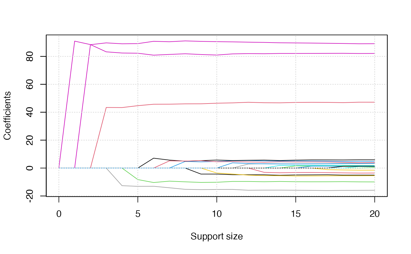
plot(abess_fit)
 plot(abess_fit, type = "tune")
 ################ logistic model ################
dataset <- generate.data(n, p, support.size, family = "binomial")
## allow cross-validation to tuning
abess_fit <- abess(dataset[["x"]], dataset[["y"]],
family = "binomial", tune.type = "cv"
)
abess_fit
#> Call:
#> abess.default(x = dataset[["x"]], y = dataset[["y"]], family = "binomial",
#> tune.type = "cv")
#>
#> support.size dev cv
#> 1 0 68.5929800 13.888785
#> 2 1 46.6936375 9.467560
#> 3 2 22.3141723 4.795585
#> 4 3 17.6033381 5.453335
#> 5 4 16.8661842 9.347666
#> 6 5 16.1567523 14.520950
#> 7 6 15.1597900 22.506390
#> 8 7 14.1855894 37.171158
#> 9 8 12.9185012 47.062152
#> 10 9 11.0144647 54.975814
#> 11 10 12.0662413 60.199527
#> 12 11 10.4759853 70.803152
#> 13 12 9.2660175 80.517063
#> 14 13 3.8066489 86.359262
#> 15 14 3.6176817 89.695262
#> 16 15 0.8178666 91.826185
#> 17 16 0.6077557 93.099175
#> 18 17 0.5993617 93.466494
#> 19 18 0.2749951 93.663214
#> 20 19 0.1004884 93.783417
#> 21 20 1.8082868 94.035446
################ poisson model ################
dataset <- generate.data(n, p, support.size, family = "poisson")
abess_fit <- abess(dataset[["x"]], dataset[["y"]],
family = "poisson", tune.type = "cv"
)
abess_fit
#> Call:
#> abess.default(x = dataset[["x"]], y = dataset[["y"]], family = "poisson",
#> tune.type = "cv")
#>
#> support.size dev cv
#> 1 0 44.95340 10.19365
#> 2 1 -31.62397 3.28437
#> 3 2 -100.57515 -10.57293
#> 4 3 -157.18472 -30.45472
#> 5 4 -160.75596 -31.01768
#> 6 5 -163.01916 -30.63952
#> 7 6 -164.82977 -30.14524
#> 8 7 -166.39686 -26.74170
#> 9 8 -167.33059 -27.33824
#> 10 9 -168.30048 -27.42207
#> 11 10 -168.98526 -27.25689
#> 12 11 -169.76250 -26.64814
#> 13 12 -170.25995 -27.38532
#> 14 13 -171.31745 -28.11082
#> 15 14 -171.54370 -28.38133
#> 16 15 -171.74975 -28.63384
#> 17 16 -171.85325 -28.08692
#> 18 17 -171.91807 -27.93900
#> 19 18 -171.94049 -28.14633
#> 20 19 -171.95597 -27.96296
#> 21 20 -171.95939 -27.89870
################ Cox model ################
dataset <- generate.data(n, p, support.size, family = "cox")
abess_fit <- abess(dataset[["x"]], dataset[["y"]],
family = "cox", tune.type = "cv"
)
################ Multivariate gaussian model ################
dataset <- generate.data(n, p, support.size, family = "mgaussian")
abess_fit <- abess(dataset[["x"]], dataset[["y"]],
family = "mgaussian", tune.type = "cv"
)
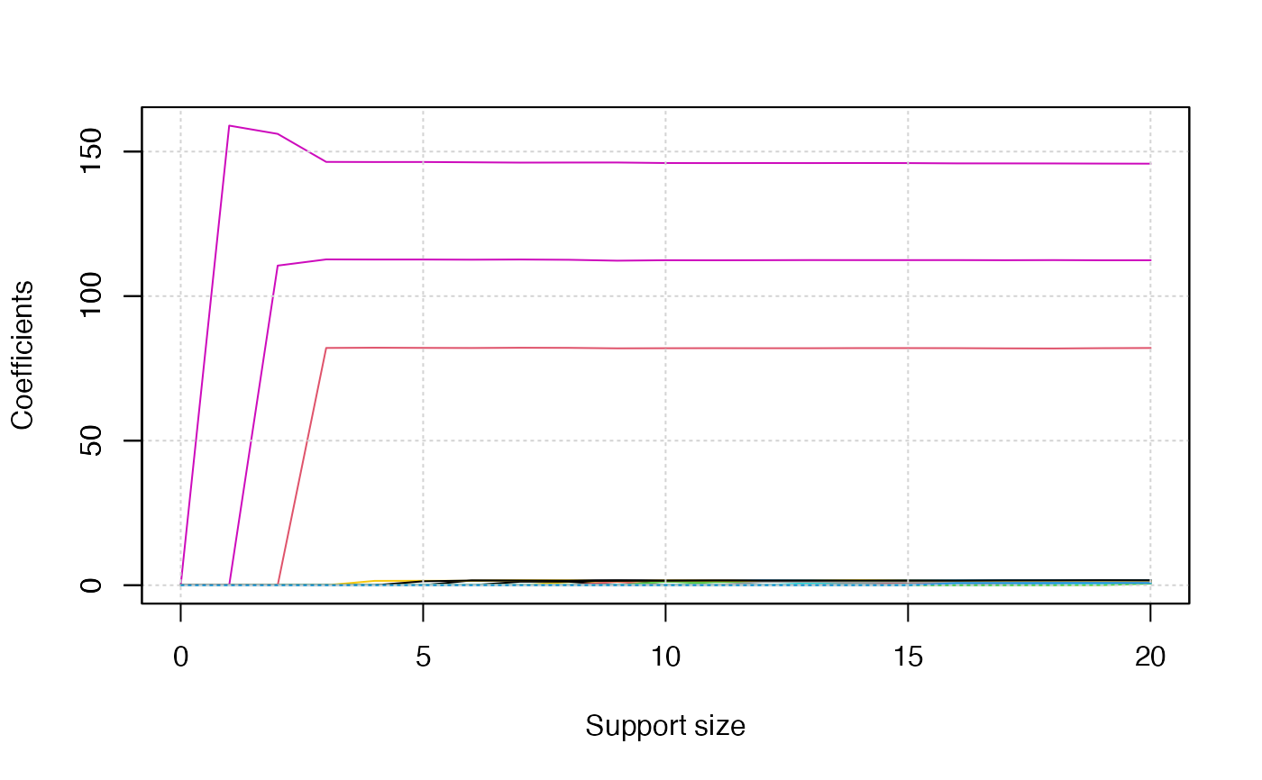
plot(abess_fit, type = "l2norm")
################ logistic model ################
dataset <- generate.data(n, p, support.size, family = "binomial")
## allow cross-validation to tuning
abess_fit <- abess(dataset[["x"]], dataset[["y"]],
family = "binomial", tune.type = "cv"
)
abess_fit
#> Call:
#> abess.default(x = dataset[["x"]], y = dataset[["y"]], family = "binomial",
#> tune.type = "cv")
#>
#> support.size dev cv
#> 1 0 68.5929800 13.888785
#> 2 1 46.6936375 9.467560
#> 3 2 22.3141723 4.795585
#> 4 3 17.6033381 5.453335
#> 5 4 16.8661842 9.347666
#> 6 5 16.1567523 14.520950
#> 7 6 15.1597900 22.506390
#> 8 7 14.1855894 37.171158
#> 9 8 12.9185012 47.062152
#> 10 9 11.0144647 54.975814
#> 11 10 12.0662413 60.199527
#> 12 11 10.4759853 70.803152
#> 13 12 9.2660175 80.517063
#> 14 13 3.8066489 86.359262
#> 15 14 3.6176817 89.695262
#> 16 15 0.8178666 91.826185
#> 17 16 0.6077557 93.099175
#> 18 17 0.5993617 93.466494
#> 19 18 0.2749951 93.663214
#> 20 19 0.1004884 93.783417
#> 21 20 1.8082868 94.035446
################ poisson model ################
dataset <- generate.data(n, p, support.size, family = "poisson")
abess_fit <- abess(dataset[["x"]], dataset[["y"]],
family = "poisson", tune.type = "cv"
)
abess_fit
#> Call:
#> abess.default(x = dataset[["x"]], y = dataset[["y"]], family = "poisson",
#> tune.type = "cv")
#>
#> support.size dev cv
#> 1 0 44.95340 10.19365
#> 2 1 -31.62397 3.28437
#> 3 2 -100.57515 -10.57293
#> 4 3 -157.18472 -30.45472
#> 5 4 -160.75596 -31.01768
#> 6 5 -163.01916 -30.63952
#> 7 6 -164.82977 -30.14524
#> 8 7 -166.39686 -26.74170
#> 9 8 -167.33059 -27.33824
#> 10 9 -168.30048 -27.42207
#> 11 10 -168.98526 -27.25689
#> 12 11 -169.76250 -26.64814
#> 13 12 -170.25995 -27.38532
#> 14 13 -171.31745 -28.11082
#> 15 14 -171.54370 -28.38133
#> 16 15 -171.74975 -28.63384
#> 17 16 -171.85325 -28.08692
#> 18 17 -171.91807 -27.93900
#> 19 18 -171.94049 -28.14633
#> 20 19 -171.95597 -27.96296
#> 21 20 -171.95939 -27.89870
################ Cox model ################
dataset <- generate.data(n, p, support.size, family = "cox")
abess_fit <- abess(dataset[["x"]], dataset[["y"]],
family = "cox", tune.type = "cv"
)
################ Multivariate gaussian model ################
dataset <- generate.data(n, p, support.size, family = "mgaussian")
abess_fit <- abess(dataset[["x"]], dataset[["y"]],
family = "mgaussian", tune.type = "cv"
)
plot(abess_fit, type = "l2norm")
 ################ Multinomial model (multi-classification) ################
dataset <- generate.data(n, p, support.size, family = "multinomial")
abess_fit <- abess(dataset[["x"]], dataset[["y"]],
family = "multinomial", tune.type = "cv"
)
predict(abess_fit,
newx = dataset[["x"]][1:10, ],
support.size = c(3, 4), type = "response"
)
#> $`3`
#> 1 2
#> [1,] 3.195041e-01 6.796433e-01 8.526063e-04
#> [2,] 9.926808e-01 2.440578e-07 7.318950e-03
#> [3,] 1.994159e-08 1.143617e-05 9.999885e-01
#> [4,] 1.922364e-09 1.000000e+00 1.508214e-08
#> [5,] 9.983972e-01 1.643894e-08 1.602810e-03
#> [6,] 4.380700e-01 4.031365e-01 1.587936e-01
#> [7,] 1.752119e-05 6.737502e-01 3.262323e-01
#> [8,] 1.397077e-06 9.834318e-01 1.656678e-02
#> [9,] 2.634263e-04 1.642880e-01 8.354486e-01
#> [10,] 5.926216e-03 2.231685e-07 9.940736e-01
#>
#> $`4`
#> 1 2
#> [1,] 1.483045e-01 8.516878e-01 7.775763e-06
#> [2,] 9.997506e-01 1.127463e-06 2.482974e-04
#> [3,] 5.750486e-11 3.022432e-09 1.000000e+00
#> [4,] 3.633381e-11 1.000000e+00 7.527000e-13
#> [5,] 9.911483e-01 5.629530e-10 8.851709e-03
#> [6,] 5.815431e-01 1.173096e-01 3.011473e-01
#> [7,] 3.581466e-06 2.443225e-02 9.755642e-01
#> [8,] 9.682266e-07 9.846618e-01 1.533721e-02
#> [9,] 2.219851e-04 7.084184e-01 2.913596e-01
#> [10,] 2.934244e-03 1.071362e-07 9.970656e-01
#>
################ Ordinal regression ################
dataset <- generate.data(n, p, support.size, family = "ordinal", class.num = 4)
abess_fit <- abess(dataset[["x"]], dataset[["y"]],
family = "ordinal", tune.type = "cv"
)
coef <- coef(abess_fit, support.size = abess_fit[["best.size"]])[[1]]
predict(abess_fit,
newx = dataset[["x"]][1:10, ],
support.size = c(3, 4), type = "response"
)
#> $`3`
#> 1 2 3
#> [1,] 4.262225e-05 1.829633e-02 9.726829e-01 8.978109e-03
#> [2,] 7.882173e-01 2.111701e-01 6.125573e-04 1.037531e-07
#> [3,] 1.486210e-05 6.456936e-03 9.682043e-01 2.532388e-02
#> [4,] 1.577722e-10 6.899165e-08 4.083410e-04 9.995916e-01
#> [5,] 9.999979e-01 2.067605e-06 4.727471e-09 8.002488e-13
#> [6,] 9.966919e-01 3.300482e-03 7.571409e-06 1.281646e-09
#> [7,] 8.368720e-10 3.659527e-07 2.162164e-03 9.978375e-01
#> [8,] 4.271390e-07 1.867472e-04 5.250122e-01 4.748006e-01
#> [9,] 8.728258e-01 1.268418e-01 3.322732e-04 5.626364e-08
#> [10,] 2.426574e-02 8.916995e-01 8.401922e-02 1.552701e-05
#>
#> $`4`
#> 1 2 3
#> [1,] 2.718879e-07 1.668930e-03 9.974270e-01 9.038274e-04
#> [2,] 9.222029e-01 7.778339e-02 1.371784e-05 2.074940e-11
#> [3,] 2.028760e-07 1.245842e-03 9.975430e-01 1.210908e-03
#> [4,] 4.080690e-15 2.509040e-11 1.659043e-05 9.999834e-01
#> [5,] 1.000000e+00 2.518530e-09 4.096723e-13 0.000000e+00
#> [6,] 9.985539e-01 1.445840e-03 2.354909e-07 3.561595e-13
#> [7,] 1.450164e-14 8.916432e-11 5.895529e-05 9.999410e-01
#> [8,] 8.009007e-10 4.924368e-06 7.650435e-01 2.349516e-01
#> [9,] 8.676204e-01 1.323548e-01 2.481049e-05 3.752842e-11
#> [10,] 4.631050e-03 9.615982e-01 3.377066e-02 5.286555e-08
#>
########## Best group subset selection #############
dataset <- generate.data(n, p, support.size)
group_index <- rep(1:10, each = 2)
abess_fit <- abess(dataset[["x"]], dataset[["y"]], group.index = group_index)
str(extract(abess_fit))
#> List of 7
#> $ beta :Formal class 'dgCMatrix' [package "Matrix"] with 6 slots
#> .. ..@ i : int [1:8] 4 5 12 13 14 15 16 17
#> .. ..@ p : int [1:2] 0 8
#> .. ..@ Dim : int [1:2] 20 1
#> .. ..@ Dimnames:List of 2
#> .. .. ..$ : chr [1:20] "x1" "x2" "x3" "x4" ...
#> .. .. ..$ : chr "4"
#> .. ..@ x : num [1:8] 1.992 82.397 -0.735 88.545 -4.368 ...
#> .. ..@ factors : list()
#> $ intercept : num -4.07
#> $ support.size: int 4
#> $ support.vars: chr [1:8] "x5" "x6" "x13" "x14" ...
#> $ support.beta: num [1:8] 1.992 82.397 -0.735 88.545 -4.368 ...
#> $ dev : num 819
#> $ tune.value : num 699
################ Golden section searching ################
dataset <- generate.data(n, p, support.size)
abess_fit <- abess(dataset[["x"]], dataset[["y"]], tune.path = "gsection")
abess_fit
#> Call:
#> abess.default(x = dataset[["x"]], y = dataset[["y"]], tune.path = "gsection")
#>
#> support.size dev GIC
#> 1 3 921.3726 696.3115
#> 2 4 833.5074 690.8643
#> 3 5 797.0079 690.9616
#> 4 6 771.9370 692.3404
#> 5 8 750.0559 698.6149
#> 6 13 722.1120 717.6933
################ Feature screening ################
p <- 1000
dataset <- generate.data(n, p, support.size)
abess_fit <- abess(dataset[["x"]], dataset[["y"]],
screening.num = 100
)
str(extract(abess_fit))
#> List of 7
#> $ beta :Formal class 'dgCMatrix' [package "Matrix"] with 6 slots
#> .. ..@ i : int [1:3] 288 642 780
#> .. ..@ p : int [1:2] 0 3
#> .. ..@ Dim : int [1:2] 1000 1
#> .. ..@ Dimnames:List of 2
#> .. .. ..$ : chr [1:1000] "x1" "x2" "x3" "x4" ...
#> .. .. ..$ : chr "3"
#> .. ..@ x : num [1:3] 145.3 51.9 160.1
#> .. ..@ factors : list()
#> $ intercept : num 5.53
#> $ support.size: int 3
#> $ support.vars: chr [1:3] "x289" "x643" "x781"
#> $ support.beta: num [1:3] 145.3 51.9 160.1
#> $ dev : num 1821
#> $ tune.value : num 772
################ Sparse predictor ################
require(Matrix)
#> Loading required package: Matrix
p <- 1000
dataset <- generate.data(n, p, support.size)
dataset[["x"]][abs(dataset[["x"]]) < 1] <- 0
dataset[["x"]] <- Matrix(dataset[["x"]])
abess_fit <- abess(dataset[["x"]], dataset[["y"]])
str(extract(abess_fit))
#> List of 7
#> $ beta :Formal class 'dgCMatrix' [package "Matrix"] with 6 slots
#> .. ..@ i : int [1:2] 288 780
#> .. ..@ p : int [1:2] 0 2
#> .. ..@ Dim : int [1:2] 1000 1
#> .. ..@ Dimnames:List of 2
#> .. .. ..$ : chr [1:1000] "x1" "x2" "x3" "x4" ...
#> .. .. ..$ : chr "2"
#> .. ..@ x : num [1:2] 147 171
#> .. ..@ factors : list()
#> $ intercept : num -10.4
#> $ support.size: int 2
#> $ support.vars: chr [1:2] "x289" "x781"
#> $ support.beta: num [1:2] 147 171
#> $ dev : num 7266
#> $ tune.value : num 910
# }
# \donttest{
################ Formula interface ################
data("trim32")
abess_fit <- abess(y ~ ., data = trim32)
abess_fit
#> Call:
#> abess.formula(formula = y ~ ., data = trim32)
#>
#> support.size dev GIC
#> 1 0 0.010369311 -548.2686
#> 2 1 0.004088476 -650.2178
#> 3 2 0.002961921 -679.1658
#> 4 3 0.002560296 -686.9195
#> 5 4 0.002392097 -685.3417
#> 6 5 0.002392089 -675.6100
#> 7 6 0.002300641 -670.5554
#> 8 7 0.002295887 -661.0715
#> 9 8 0.002275372 -652.4165
#> 10 9 0.002275332 -642.6865
#> 11 10 0.002256348 -633.9598
#> 12 11 0.002243761 -624.8989
#> 13 12 0.002225414 -616.1521
# }
################ Multinomial model (multi-classification) ################
dataset <- generate.data(n, p, support.size, family = "multinomial")
abess_fit <- abess(dataset[["x"]], dataset[["y"]],
family = "multinomial", tune.type = "cv"
)
predict(abess_fit,
newx = dataset[["x"]][1:10, ],
support.size = c(3, 4), type = "response"
)
#> $`3`
#> 1 2
#> [1,] 3.195041e-01 6.796433e-01 8.526063e-04
#> [2,] 9.926808e-01 2.440578e-07 7.318950e-03
#> [3,] 1.994159e-08 1.143617e-05 9.999885e-01
#> [4,] 1.922364e-09 1.000000e+00 1.508214e-08
#> [5,] 9.983972e-01 1.643894e-08 1.602810e-03
#> [6,] 4.380700e-01 4.031365e-01 1.587936e-01
#> [7,] 1.752119e-05 6.737502e-01 3.262323e-01
#> [8,] 1.397077e-06 9.834318e-01 1.656678e-02
#> [9,] 2.634263e-04 1.642880e-01 8.354486e-01
#> [10,] 5.926216e-03 2.231685e-07 9.940736e-01
#>
#> $`4`
#> 1 2
#> [1,] 1.483045e-01 8.516878e-01 7.775763e-06
#> [2,] 9.997506e-01 1.127463e-06 2.482974e-04
#> [3,] 5.750486e-11 3.022432e-09 1.000000e+00
#> [4,] 3.633381e-11 1.000000e+00 7.527000e-13
#> [5,] 9.911483e-01 5.629530e-10 8.851709e-03
#> [6,] 5.815431e-01 1.173096e-01 3.011473e-01
#> [7,] 3.581466e-06 2.443225e-02 9.755642e-01
#> [8,] 9.682266e-07 9.846618e-01 1.533721e-02
#> [9,] 2.219851e-04 7.084184e-01 2.913596e-01
#> [10,] 2.934244e-03 1.071362e-07 9.970656e-01
#>
################ Ordinal regression ################
dataset <- generate.data(n, p, support.size, family = "ordinal", class.num = 4)
abess_fit <- abess(dataset[["x"]], dataset[["y"]],
family = "ordinal", tune.type = "cv"
)
coef <- coef(abess_fit, support.size = abess_fit[["best.size"]])[[1]]
predict(abess_fit,
newx = dataset[["x"]][1:10, ],
support.size = c(3, 4), type = "response"
)
#> $`3`
#> 1 2 3
#> [1,] 4.262225e-05 1.829633e-02 9.726829e-01 8.978109e-03
#> [2,] 7.882173e-01 2.111701e-01 6.125573e-04 1.037531e-07
#> [3,] 1.486210e-05 6.456936e-03 9.682043e-01 2.532388e-02
#> [4,] 1.577722e-10 6.899165e-08 4.083410e-04 9.995916e-01
#> [5,] 9.999979e-01 2.067605e-06 4.727471e-09 8.002488e-13
#> [6,] 9.966919e-01 3.300482e-03 7.571409e-06 1.281646e-09
#> [7,] 8.368720e-10 3.659527e-07 2.162164e-03 9.978375e-01
#> [8,] 4.271390e-07 1.867472e-04 5.250122e-01 4.748006e-01
#> [9,] 8.728258e-01 1.268418e-01 3.322732e-04 5.626364e-08
#> [10,] 2.426574e-02 8.916995e-01 8.401922e-02 1.552701e-05
#>
#> $`4`
#> 1 2 3
#> [1,] 2.718879e-07 1.668930e-03 9.974270e-01 9.038274e-04
#> [2,] 9.222029e-01 7.778339e-02 1.371784e-05 2.074940e-11
#> [3,] 2.028760e-07 1.245842e-03 9.975430e-01 1.210908e-03
#> [4,] 4.080690e-15 2.509040e-11 1.659043e-05 9.999834e-01
#> [5,] 1.000000e+00 2.518530e-09 4.096723e-13 0.000000e+00
#> [6,] 9.985539e-01 1.445840e-03 2.354909e-07 3.561595e-13
#> [7,] 1.450164e-14 8.916432e-11 5.895529e-05 9.999410e-01
#> [8,] 8.009007e-10 4.924368e-06 7.650435e-01 2.349516e-01
#> [9,] 8.676204e-01 1.323548e-01 2.481049e-05 3.752842e-11
#> [10,] 4.631050e-03 9.615982e-01 3.377066e-02 5.286555e-08
#>
########## Best group subset selection #############
dataset <- generate.data(n, p, support.size)
group_index <- rep(1:10, each = 2)
abess_fit <- abess(dataset[["x"]], dataset[["y"]], group.index = group_index)
str(extract(abess_fit))
#> List of 7
#> $ beta :Formal class 'dgCMatrix' [package "Matrix"] with 6 slots
#> .. ..@ i : int [1:8] 4 5 12 13 14 15 16 17
#> .. ..@ p : int [1:2] 0 8
#> .. ..@ Dim : int [1:2] 20 1
#> .. ..@ Dimnames:List of 2
#> .. .. ..$ : chr [1:20] "x1" "x2" "x3" "x4" ...
#> .. .. ..$ : chr "4"
#> .. ..@ x : num [1:8] 1.992 82.397 -0.735 88.545 -4.368 ...
#> .. ..@ factors : list()
#> $ intercept : num -4.07
#> $ support.size: int 4
#> $ support.vars: chr [1:8] "x5" "x6" "x13" "x14" ...
#> $ support.beta: num [1:8] 1.992 82.397 -0.735 88.545 -4.368 ...
#> $ dev : num 819
#> $ tune.value : num 699
################ Golden section searching ################
dataset <- generate.data(n, p, support.size)
abess_fit <- abess(dataset[["x"]], dataset[["y"]], tune.path = "gsection")
abess_fit
#> Call:
#> abess.default(x = dataset[["x"]], y = dataset[["y"]], tune.path = "gsection")
#>
#> support.size dev GIC
#> 1 3 921.3726 696.3115
#> 2 4 833.5074 690.8643
#> 3 5 797.0079 690.9616
#> 4 6 771.9370 692.3404
#> 5 8 750.0559 698.6149
#> 6 13 722.1120 717.6933
################ Feature screening ################
p <- 1000
dataset <- generate.data(n, p, support.size)
abess_fit <- abess(dataset[["x"]], dataset[["y"]],
screening.num = 100
)
str(extract(abess_fit))
#> List of 7
#> $ beta :Formal class 'dgCMatrix' [package "Matrix"] with 6 slots
#> .. ..@ i : int [1:3] 288 642 780
#> .. ..@ p : int [1:2] 0 3
#> .. ..@ Dim : int [1:2] 1000 1
#> .. ..@ Dimnames:List of 2
#> .. .. ..$ : chr [1:1000] "x1" "x2" "x3" "x4" ...
#> .. .. ..$ : chr "3"
#> .. ..@ x : num [1:3] 145.3 51.9 160.1
#> .. ..@ factors : list()
#> $ intercept : num 5.53
#> $ support.size: int 3
#> $ support.vars: chr [1:3] "x289" "x643" "x781"
#> $ support.beta: num [1:3] 145.3 51.9 160.1
#> $ dev : num 1821
#> $ tune.value : num 772
################ Sparse predictor ################
require(Matrix)
#> Loading required package: Matrix
p <- 1000
dataset <- generate.data(n, p, support.size)
dataset[["x"]][abs(dataset[["x"]]) < 1] <- 0
dataset[["x"]] <- Matrix(dataset[["x"]])
abess_fit <- abess(dataset[["x"]], dataset[["y"]])
str(extract(abess_fit))
#> List of 7
#> $ beta :Formal class 'dgCMatrix' [package "Matrix"] with 6 slots
#> .. ..@ i : int [1:2] 288 780
#> .. ..@ p : int [1:2] 0 2
#> .. ..@ Dim : int [1:2] 1000 1
#> .. ..@ Dimnames:List of 2
#> .. .. ..$ : chr [1:1000] "x1" "x2" "x3" "x4" ...
#> .. .. ..$ : chr "2"
#> .. ..@ x : num [1:2] 147 171
#> .. ..@ factors : list()
#> $ intercept : num -10.4
#> $ support.size: int 2
#> $ support.vars: chr [1:2] "x289" "x781"
#> $ support.beta: num [1:2] 147 171
#> $ dev : num 7266
#> $ tune.value : num 910
# }
# \donttest{
################ Formula interface ################
data("trim32")
abess_fit <- abess(y ~ ., data = trim32)
abess_fit
#> Call:
#> abess.formula(formula = y ~ ., data = trim32)
#>
#> support.size dev GIC
#> 1 0 0.010369311 -548.2686
#> 2 1 0.004088476 -650.2178
#> 3 2 0.002961921 -679.1658
#> 4 3 0.002560296 -686.9195
#> 5 4 0.002392097 -685.3417
#> 6 5 0.002392089 -675.6100
#> 7 6 0.002300641 -670.5554
#> 8 7 0.002295887 -661.0715
#> 9 8 0.002275372 -652.4165
#> 10 9 0.002275332 -642.6865
#> 11 10 0.002256348 -633.9598
#> 12 11 0.002243761 -624.8989
#> 13 12 0.002225414 -616.1521
# }