Adaptive best subset selection for principal component analysis
abesspca(
  x,
  type = c("predictor", "gram"),
  sparse.type = c("fpc", "kpc"),
  cor = FALSE,
  kpc.num = NULL,
  support.size = NULL,
  gs.range = NULL,
  tune.path = c("sequence", "gsection"),
  tune.type = c("gic", "aic", "bic", "ebic", "cv"),
  nfolds = 5,
  foldid = NULL,
  ic.scale = 1,
  c.max = NULL,
  always.include = NULL,
  group.index = NULL,
  screening.num = NULL,
  splicing.type = 1,
  max.splicing.iter = 20,
  warm.start = TRUE,
  num.threads = 0,
  ...
)
Arguments
- x
A matrix object. It can be either a predictor matrix where each row is an observation and each column is a predictor or a sample covariance/correlation matrix. If
xis a predictor matrix, it can be in sparse matrix format (inherit from class"dgCMatrix"in packageMatrix).- type
If
type = "predictor",xis considered as the predictor matrix. Iftype = "gram",xis considered as a sample covariance or correlation matrix.- sparse.type
If
sparse.type = "fpc", then best subset selection performs on the first principal component; Ifsparse.type = "kpc", then best subset selection would be sequentially performed on the firstkpc.numnumber of principal components. Ifkpc.numis supplied, the default issparse.type = "kpc"; otherwise, issparse.type = "fpc".- cor
A logical value. If
cor = TRUE, perform PCA on the correlation matrix; otherwise, the covariance matrix. This option is available only iftype = "predictor". Default:cor = FALSE.- kpc.num
A integer decide the number of principal components to be sequentially considered.
- support.size
It is a flexible input. If it is an integer vector. It represents the support sizes to be considered for each principal component. If it is a
listobject containingkpc.numnumber of integer vectors, the i-th principal component consider the support size specified in the i-th element in thelist. Only used fortune.path = "sequence". The default issupport.size = NULL, and some rules in details section are used to specifysupport.size.- gs.range
A integer vector with two elements. The first element is the minimum model size considered by golden-section, the later one is the maximum one. Default is
gs.range = c(1, min(n, round(n/(log(log(n))log(p))))).- tune.path
The method to be used to select the optimal support size. For
tune.path = "sequence", we solve the best subset selection problem for each size insupport.size. Fortune.path = "gsection", we solve the best subset selection problem with support size ranged ings.range, where the specific support size to be considered is determined by golden section.- tune.type
The type of criterion for choosing the support size. Available options are
"gic","ebic","bic","aic"and"cv". Default is"gic".tune.type = "cv"is available only whentype = "predictor".- nfolds
The number of folds in cross-validation. Default is
nfolds = 5.- foldid
an optional integer vector of values between 1, ..., nfolds identifying what fold each observation is in. The default
foldid = NULLwould generate a random foldid.- ic.scale
A non-negative value used for multiplying the penalty term in information criterion. Default:
ic.scale = 1.- c.max
an integer splicing size. The default of
c.maxis the maximum of 2 andmax(support.size) / 2.- always.include
An integer vector containing the indexes of variables that should always be included in the model.
- group.index
A vector of integers indicating the which group each variable is in. For variables in the same group, they should be located in adjacent columns of
xand their corresponding index ingroup.indexshould be the same. Denote the first group as1, the second2, etc. If you do not fit a model with a group structure, please setgroup.index = NULL(the default).- screening.num
An integer number. Preserve
screening.numnumber of predictors with the largest marginal maximum likelihood estimator before running algorithm.- splicing.type
Optional type for splicing. If
splicing.type = 1, the number of variables to be spliced isc.max, ...,1; ifsplicing.type = 2, the number of variables to be spliced isc.max,c.max/2, ...,1. Default:splicing.type = 1.- max.splicing.iter
The maximum number of performing splicing algorithm. In most of the case, only a few times of splicing iteration can guarantee the convergence. Default is
max.splicing.iter = 20.- warm.start
Whether to use the last solution as a warm start. Default is
warm.start = TRUE.- num.threads
An integer decide the number of threads to be concurrently used for cross-validation (i.e.,
tune.type = "cv"). Ifnum.threads = 0, then all of available cores will be used. Default:num.threads = 0.- ...
further arguments to be passed to or from methods.
Value
A S3 abesspca class object, which is a list with the following components:
- coef
A \(p\)-by-
length(support.size)loading matrix of sparse principal components (PC), where each row is a variable and each column is a support size;- nvars
The number of variables.
- sparse.type
The same as input.
- support.size
The actual support.size values used. Note that it is not necessary the same as the input if the later have non-integer values or duplicated values.
- ev
A vector with size
length(support.size). It records the cumulative sums of explained variance at each support size.- tune.value
A value of tuning criterion of length
length(support.size).- kpc.num
The number of principal component being considered.
- var.pc
The variance of principal components obtained by performing standard PCA.
- cum.var.pc
Cumulative sums of
var.pc.- var.all
If
sparse.type = "fpc", it is the total standard deviations of all principal components.- pev
A vector with the same length as
ev. It records the percent of explained variance (compared tovar.all) at each support size.- pev.pc
It records the percent of explained variance (compared to
var.pc) at each support size.- tune.type
The criterion type for tuning parameters.
- tune.path
The strategy for tuning parameters.
- call
The original call to
abess.
It is worthy to note that, if sparse.type == "kpc", the coef, support.size, ev, tune.value, pev and pev.pc in list are list objects.
Details
Adaptive best subset selection for principal component analysis (abessPCA) aim
to solve the non-convex optimization problem:
$$-\arg\min_{v} v^\top \Sigma v, s.t.\quad v^\top v=1, \|v\|_0 \leq s, $$
where \(s\) is support size.
Here, \(\Sigma\) is covariance matrix, i.e.,
$$\Sigma = \frac{1}{n} X^{\top} X.$$
A generic splicing technique is implemented to
solve this problem.
By exploiting the warm-start initialization, the non-convex optimization
problem at different support size (specified by support.size)
can be efficiently solved.
The abessPCA can be conduct sequentially for each component.
Please see the multiple principal components Section on the website
for more details about this function.
For abesspca function, the arguments kpc.num control the number of components to be consider.
When sparse.type = "fpc" but support.size is not supplied,
it is set as support.size = 1:min(ncol(x), 100) if group.index = NULL;
otherwise, support.size = 1:min(length(unique(group.index)), 100).
When sparse.type = "kpc" but support.size is not supplied,
then for 20\
it is set as min(ncol(x), 100) if group.index = NULL;
otherwise, min(length(unique(group.index)), 100).
Note
Some parameters not described in the Details Section is explained in the document for abess
because the meaning of these parameters are very similar.
References
A polynomial algorithm for best-subset selection problem. Junxian Zhu, Canhong Wen, Jin Zhu, Heping Zhang, Xueqin Wang. Proceedings of the National Academy of Sciences Dec 2020, 117 (52) 33117-33123; doi:10.1073/pnas.2014241117
Sparse principal component analysis. Hui Zou, Hastie Trevor, and Tibshirani Robert. Journal of computational and graphical statistics 15.2 (2006): 265-286. doi:10.1198/106186006X113430
See also
Examples
# \donttest{
library(abess)
Sys.setenv("OMP_THREAD_LIMIT" = 2)
## predictor matrix input:
head(USArrests)
#> Murder Assault UrbanPop Rape
#> Alabama 13.2 236 58 21.2
#> Alaska 10.0 263 48 44.5
#> Arizona 8.1 294 80 31.0
#> Arkansas 8.8 190 50 19.5
#> California 9.0 276 91 40.6
#> Colorado 7.9 204 78 38.7
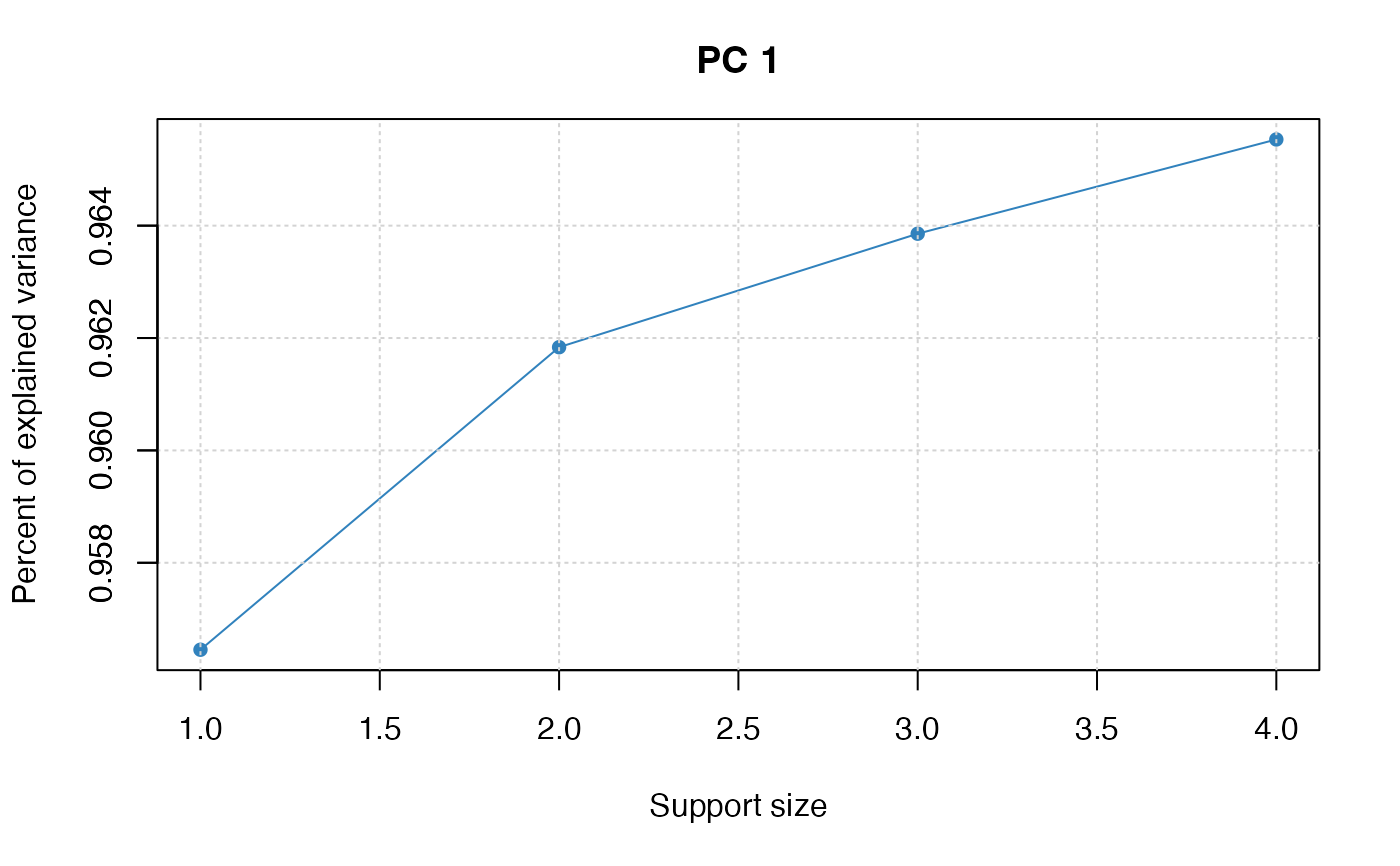
pca_fit <- abesspca(USArrests)
pca_fit
#> Call:
#> abesspca(x = USArrests)
#>
#> PC support.size ev pev
#> 1 1 1 6806.262 0.9564520
#> 2 1 2 6844.578 0.9618364
#> 3 1 3 6858.954 0.9638565
#> 4 1 4 6870.893 0.9655342
plot(pca_fit)
 ## covariance matrix input:
cov_mat <- stats::cov(USArrests) * (nrow(USArrests) - 1) / nrow(USArrests)
pca_fit <- abesspca(cov_mat, type = "gram")
pca_fit
#> Call:
#> abesspca(x = cov_mat, type = "gram")
#>
#> PC support.size ev pev
#> 1 1 1 6806.262 0.9564520
#> 2 1 2 6844.578 0.9618364
#> 3 1 3 6858.954 0.9638565
#> 4 1 4 6870.893 0.9655342
## robust covariance matrix input:
rob_cov <- MASS::cov.rob(USArrests)[["cov"]]
rob_cov <- (rob_cov + t(rob_cov)) / 2
pca_fit <- abesspca(rob_cov, type = "gram")
pca_fit
#> Call:
#> abesspca(x = rob_cov, type = "gram")
#>
#> PC support.size ev pev
#> 1 1 1 6515.015 0.9627318
#> 2 1 2 6547.268 0.9674980
#> 3 1 3 6577.429 0.9719548
#> 4 1 4 6588.893 0.9736488
## K-component principal component analysis
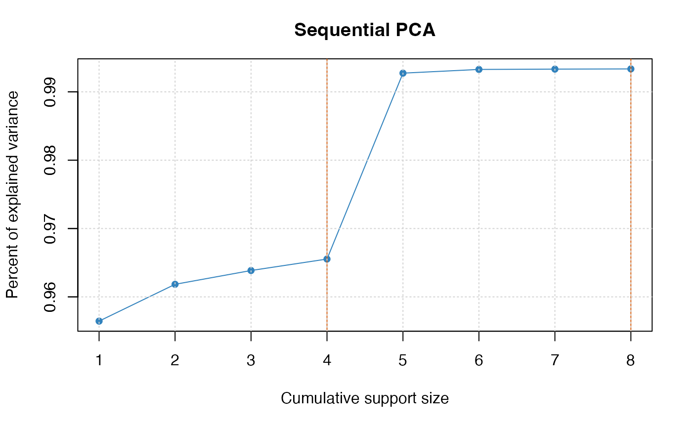
pca_fit <- abesspca(USArrests,
sparse.type = "kpc",
support.size = 1:4
)
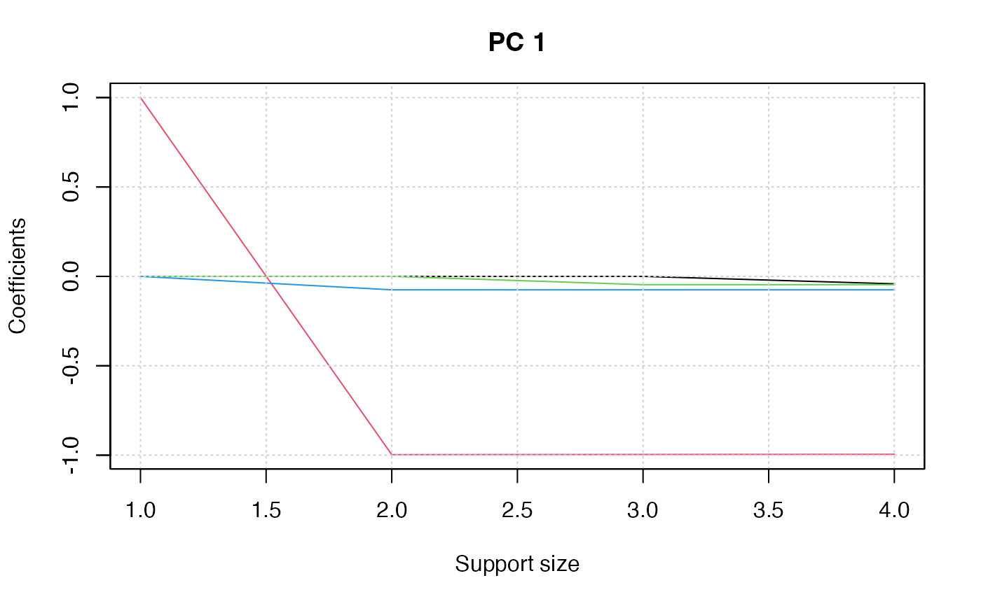
coef(pca_fit)
#> [[1]]
#> 4 x 4 sparse Matrix of class "dgCMatrix"
#> 1 2 3 4
#> Murder . . . -0.04170432
#> Assault 1 -0.99717739 -0.99608572 -0.99522128
#> UrbanPop . . -0.04643219 -0.04633575
#> Rape . -0.07508168 -0.07521497 -0.07515550
#>
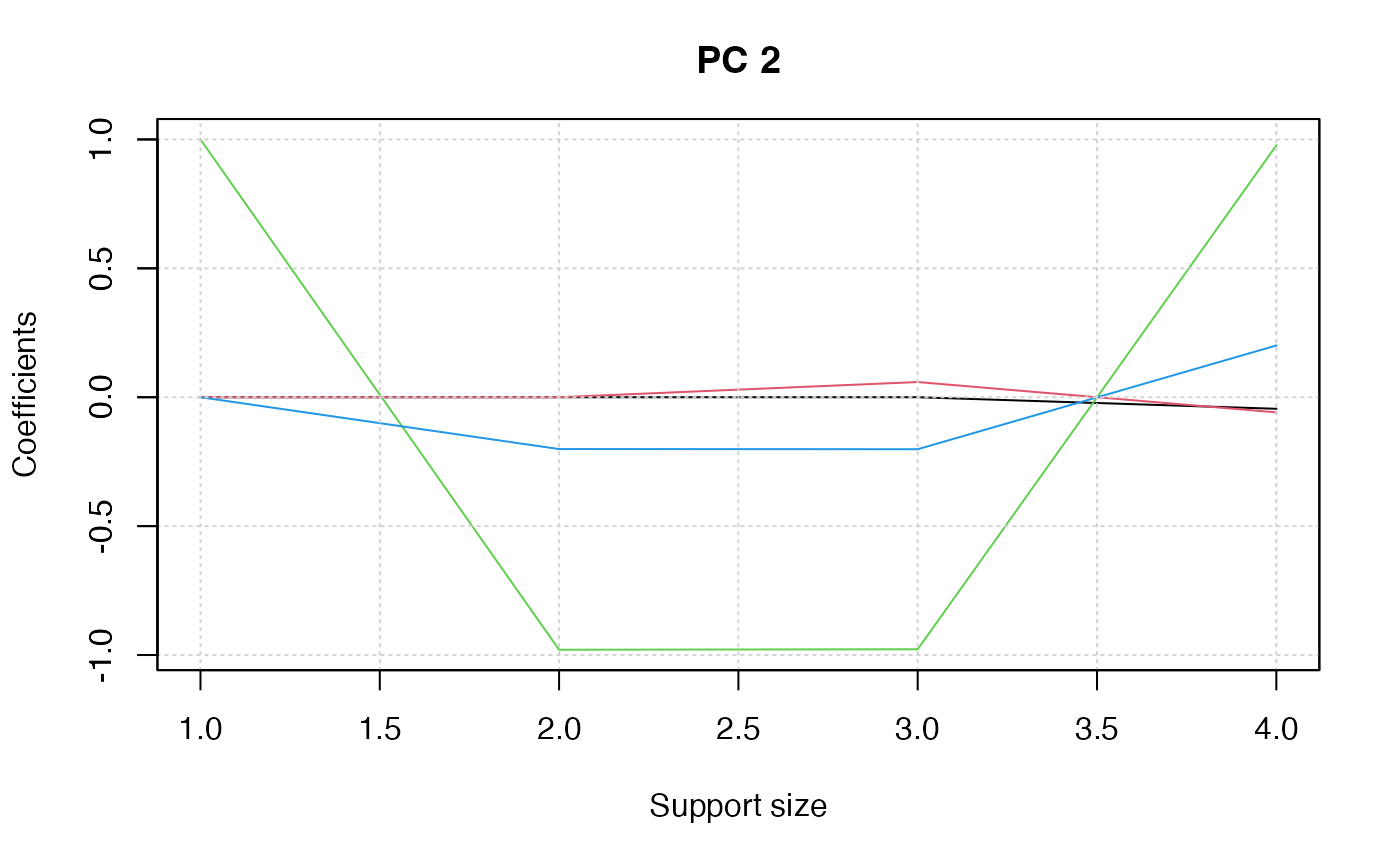
#> [[2]]
#> 4 x 4 sparse Matrix of class "dgCMatrix"
#> 1 2 3 4
#> Murder . . -0.05886581 0.05886581
#> Assault . . . .
#> UrbanPop 1 -0.9320592 -0.92786886 0.92786886
#> Rape . -0.3623060 -0.36823117 0.36823117
#>
plot(pca_fit)
 plot(pca_fit, "coef")
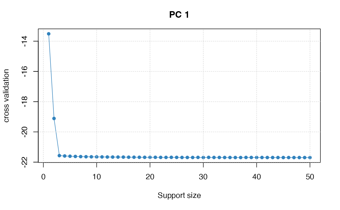
 ## select support size via cross-validation ##
n <- 500
p <- 50
support_size <- 3
dataset <- generate.spc.matrix(n, p, support_size, snr = 20)
spca_fit <- abesspca(dataset[["x"]], tune.type = "cv", nfolds = 5)
plot(spca_fit, type = "tune")
 # }
# }